|
Anthony
Pym 1999
WHO
NEEDS STATISTICS?
Research
projects in linguistics and cultural studies may or may
not need some basic statistics.
Statistics
are NOT needed when:
1. You
have no quantified data (i.e. no numbers) and you are happy
doing qualitative research
2. You
have no hypothesis to test (i.e. you’re not really doing
research)
3. You
can get all the information you need just by looking at
the relative sizes of data (in graphs, by calculating simple
averages, counting on fingers and toes or whatever) and
you thus do not need to say how strong or weak a relation
is.
Statistics
may be needed when:
1. You
want your work to look scientific
2. You
are dealing with a probabilistic hypothesis
3. You
do have to say how strong or weak a relation is, and you
can’t tell just by looking at a pie chart, a graph, or some
simple representation
4. You
have to say to what extent the relation observed cannot
be due to chance (i.e. how significant it is, or better,
how representative your sample might be).
SOME
BASIC TERMS
Hypothesis:
A proposition that can be proven true or false on the basis
of some kind of observation or testing procedure.
Probability:
The likelihood of an event occurring. If an event has never
occurred in the field observed, its probability is 0. If
it has always occurred, its probability is 1. Probability
can thus be expressed as a number between 0 and 1.
Probabilistic
hypothesis: In a very loose sense, a hypothesis of
the kind ‘when X occurs, Y will tend to occur also’, or
‘The more X, the more/less Y’, or ‘when X occurs, Y will
tend to occur more than Z’, and so on.
For
example, here is the hypothesis that we’re going to test:
‘The more recent the menu translation, the lower evaluation
it will receive from foreigners.’ (i.e. translations of
menus in restaurants are getting worse) (Fallada 1998).
This does not mean that all recent translations are bad,
nor that all old ones are good. It merely posits a tendency,
a probabilistic relationship that must be observed, quantified
on the basis of a sample, and tested to see if it is significant.
MORE
BASIC TERMS
Variable:
A feature that can be quantified. Better, a question that
can be answered in a quantitative way. In our example the
two variables are ‘date of menu translation’ and ‘evaluation
by foreigners’ (i.e. the questions ‘When was the translation
done?’, and ‘What score does the user give?’).
Data:
The numbers that quantify the variables; the actual answers
to the questions. In this case, the dates of the translations,
and the scores given by the foreigners.
Value:
Each of the actual answers (e.g. 1988, 1998, or 30, 50,
60 over 100).
TYPES
OF DATA
Nominal
data: Data that cannot be related in an ordinal way. For
example, the menus are known by the name of the restaurant
they come from, but those names are not relevant to our
research. So we codify the menus as 1, 2, 3, 4, 5, 6, 7,
and so on. These numbers are names; they are nominal data;
they cannot be compared in terms of intervals.
Continuous
or interval data: Data that are significant in an ordinal
way. When the evaluators give scores to the menus, a score
of 70 is worth more than a score of 50, and so on. It is
thus significant to compare and measure intervals.
The
difference between nominal and continuous data seems simple
enough. As indeed is talk about nominal and continous variables.
But the difference is not always quite so clear. For example,
in this research the sample included seven menus from the
1960s-1970s and seven from the 1980s-1990s. The dates could
have been treated as continuous data but it was considered
more convenient to look at the two groups of menus in terms
of ‘old’ and ‘new’, just comparing the two groups. This
meant that the dates actually became nominal data, naming
the two groups and nothing more.
MEAN
AND MEDIAN
Mean:
What everyone else calls the 'average' of a set of data.
An English girl evaluated the 14 menus as follows (scores
out of 50):
| Old |
35 |
45 |
45 |
45 |
30 |
40 |
40 |
| New |
20 |
00 |
35 |
10 |
30 |
30 |
15 |
To get
the mean we add up the scores and divide by the number of
scores. The mean of the top row (Old) is 40; the mean of
the bottom row (New) is 20. So, on average, the older menus
were considered better than the newer ones.
Median:
The middle score, when the scores are put in order. For
example, we could order the above scores as follows (it
makes no difference, since the order of presentation was
only based on nominal values anyway):
| Old |
30
|
35
|
35
|
40
|
40
|
45
|
45
|
| New |
00
|
10
|
15
|
20
|
30
|
30
|
35
|
Here
the median is 40 for OLD and 20 for NEW. So the medians
are in this case the same as the means.
Sometimes
the mean is misleading because of some anomaly in the sample.
If, for example, one of the New menus scored a maximum 50,
the mean would go up to 22.1 but the median would stay at
20. Medians are thus used as a way of reducing the effect
of these exceptional score or ‘outliers’. But it is often
just as easy and effective to delete the outliers and proceed
with means (as will be explained below).
Often
means are all you need to know about statistics. In the
case of the menus, six evaluators were used, in three pairs
of two (English-speakers with no Spanish, English-speakers
with good Spanish; German speakers with no Spanish). Means
were then used for each pair, since the differences between
them were not great. The questions concerned ‘Language’
(L) features and ‘Culture’ (C) features, so the mean scores
are presented in two blocks, as follows:
|
|
L
|
L
|
L
|
C
|
C
|
C
|
| Old |
40
|
43.5
|
37.1
|
32.8
|
37.1
|
34.2
|
| New |
20
|
27.8
|
18.6
|
16.4
|
25.0
|
15.7
|
| Difference |
20
|
15.7
|
18.5
|
16.4
|
12.1
|
18.5
|
In all cases there is a clear difference between the Old
and New menus, so there is little need to keep doing statistics
in order to test this particular hypothesis. The mean difference
for Language questions was 18.0; the mean difference for
Culture questions was 15.6. The overall mean difference
was thus 16.8 points. This is great enough to be declared
significant without any further ado.
TESTING
SIGNIFICANCE
However,
we might want to make sure that this difference is not just
due to chance. Further, we might wonder if the difference
between the Language and Culture scores was significant,
or if it is entirely by chance that the English-speaker
who know Spanish gave higher scores and made less of a difference
between the Old and the New menus. To answer these questions,
we need some kind of statistical test.
THE
NULL HYPOTHESIS
In all
these cases we have to consider the possibility that what
we think we have found is just due to chance (be it good
luck or bad luck). This ‘chance’ possibility is expressed
as the ‘null hypothesis’ (H0), which is the hypothesis that
we DON’T want to be true. Our null hypotheses would thus
be:
- The mean scores for New and Old menus are exactly the
same.
- Mean scores for Language and Culture radically different
(i.e. without correlation).
- Mean scores for all evaluators are radically different
(i.e. without correlation).
RANGE,
DISPERSION AND VARIANCE
For
our findings to be significant, the probability of them
occurring has to be greater than that of the corresponding
null hypothesis.
One
indication of that probability is how closely the scores
are grouped around their mean. If there were a lot of randomness
in our data, or if our sample were simply too small for
the phenomenon we are trying to test, the scores would wander
from high to low for both the Old and New menus, and any
difference in the means would be due to no more than luck.
We are thus interested in measuring how close the scores
are to their means.
The
range is the distance between the highest and the
lowest score. On the basis of the above numbers, the range
for Old menus is 43.5 - 32.8 = 10.7. The range for the New
menus is 27.8 - 15.7 = 12.1. So the scores for the Old menus
are more closely grouped than those for the New menus. But
this doesn’t really tell us very much.
If we
want to measure the dispersion of all the scores, and not
merely the highest and the lowest, we have to measure the
standard deviation. This measures how far all scores
are away from the mean, whether above or below the mean.
To do
this manually, you take the difference between each score
individual score and the mean, then square all those differences
(so it doesn’t matter if they’re greater than or less than
the mean), then add them up and divide by the number of
scores less one.
If you’re
smart, you just feed your scores into a computer programme
(I’m using StatView), ask the programme what the standard
deviation is, and write down the answer. In this case the
standard deviation for Old is 38.8, and for New is 48.4.
So the scores for the Old menus are still more closely grouped,
and this still doesn’t tell us very much.
BUT
THERE IS A BIG TRICK:
By looking
at how well grouped your scores are, and bearing in mind
how many scores you have (i.e. the size of your sample),
statistics can estimate the probability of those scores
representing either normal patterns or simple chance. More
technically, it is possible to assess how extreme a sample’s
mean is with respect to the distribution of means for all
possible samples.
This
makes sense. If you just have two scores and they are closely
grouped (say, 40 and 42 in our example), that grouping is
not as reliable as data with five scores and a slightly
wider range (say, 38, 40, 40, 41, 42). The significance
of the patterns we find thus depends on BOTH the grouping
of the data AND the number of items in the data. This significance
is measured in terms of the probability that the grouping
is due to chance. That probability is expressed as the value
p (or 'p-value'), which will be a number between 0 and 1
(remembering what we said about probability above).
To assess
significance, you thus either read a book on statistics
(here we are drawing on Wright 1997) or feed your data into
a computer programme (we will be using StatView and a bit
of KaleidaGraph). If you do the latter, you will usually
do something called a t-test and just look for a p-value.
If the p-value is very small (usually written as <0.001),
the significance of your data is okay (i.e. the probabilityof
the null-hypothesis is very low). If the p-value is big
(usually 0.05 or more), try something else.
The
p-value for both our groups of menus is < 0.001. So we
don’t really have much to worry about. But someone might
want to know what is going on. If so, move to the next section.
T-TESTS
FOR PAIRED DATA
T-tests
were invented by a man who used the pseudonym ‘Student’.
So they are sometimes called Student-tests. But they are
not just for students.
As mentioned,
T-tests are used to assess the statistical significance
of data. Of the several types of t-test, a paired t-test
is used to compare sets of data that are matched in some
way and we want to see if the means are different (i.e.
if there is some general significant difference between
the two sets of scores).
This
could involve comparing two variables for the same people,
as in a Before-After study (scores before a lesson vs scores
after a lesson). In these cases each of the scores in one
group corresponds to a score in the other (i.e. the same
subject, before and after) and we are hoping that there
will be a significant difference between the two means (i.e.
that all the individual subjects will have learnt something
from the lesson). The data are thus said to be paired.
In our
menu example the main variables we are interested in are
not really paired, since we have decided to treat the dates
of the menus as nominal data.
Further,
the paired data that we do have are not really suited to
a t-test. Since all the menus were evaluated for Language
and Cultural errors, for each case (each menu) we have a
Language score and a Culture score. These are indeed paired.
But we are not going to hypothesize that the means between
the two are significantly different, since there is no change
or event separating the two sets of scores. In fact, we
would hope that the scores are related in such a way that
there is either no significant difference or that when one
goes up, the other goes up (i.e. a good menu is good in
terms of both Language and Culture errors).
In these
cases we simply test for correlation/covariance, as explained
below. No t-test is necessary.
Perhaps
the only part of our example that is suitable for a paired
t-test is at the end of the research, where the worst menus
(those from the 1990s) were retranslated with the aid of
official glossaries for restaurants. These retranslatations
were then assessed by one group of informants, with clearly
better results. The scores were as follows:
|
Before
|
After
|
|
25
|
35
|
|
00
|
35
|
|
25
|
35
|
|
10
|
25
|
|
20
|
25
|
|
20
|
45
|
|
10
|
25
|
When these scores are put into StatView and a paired t-test
is applied, here is what we get:
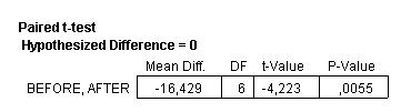
This
tells us that the difference between the means is 16.429
(the mean for the Before menus is actually 15.714; the mean
for the retranslations is 32.143). It also tells us how
big the sample is, since the DF here stands for ‘degrees
of freedom’ and actually counts the number of cases minus
one (thus, 7 menus - 1 = 6 DF). But we can get all that
by counting on our fingers.
(Don’t
ask why the number of cases is called ‘degrees of freedom’;
don’t ask why we subtract one; this is for idiots, so just
read on, okay?)
Fortunately
the test also gives us a number known as a t-value, here
4.223 (the + and - signs don’t matter, since they only depend
on what group we list first). Basically, the bigger the
t-value, the greater the difference and the happier we should
be. But life is not quite that simple. In order for our
finding to be significant, the t-value has to be greater
than the minimal t-value for the particular degrees of freedom
and threshold of significance (sometimes called an a value)
we are concerned with. Here we have a DF of 6 and our threshold
may as well be the normal 0.05 (i.e. a p-value above this
would not enable us to exclude the null hypothesis).
So,
you go to a t-table (Student’s t-distribution), go down
the df column (on the left) until you get to 6 (or whatever),
go across to the corresponding value in the 0.05 column,
and you get a number, in fact a t-value. If we are doing
a two-tailed test, that number is 2.45. That means that
our own t-value has to be greater than 2.45 if our finding
is to be significant. In fact our t-value is 4.223, so our
finding is indeed significant, and we have a right to be
happy.
Now,
you can more or less forget the previous paragraphs (if
you want to know about one-tailed and two-tailed tests,
consult a book; if you have to decide and you don’t have
a book, choose two-tailed). You can forget most of this
because our computer programme also gives us the corresponding
p-value. In this case the p-value is 0.0055. As mentioned,
to have a significant finding we generally only need a p-value
of 0.05 (expressed as ? = 0.05), although this is merely
an informal conventional threshold that could go higher
or lower as the case may be. In our case here, the p-value
is well below 0.05 so our pattern is significant and that’s
all we really need to know.
We can
then express this result as follows:
t(6)
= 4.223; p = 0.0055
And
this is exactly what you should put in your paper when you
are giving your results. We’ve given the t value (although
we are not really interested in looking it up in the tables),
we’ve given the df (in brackets), and we have given the
all-important p-value. This should impress the multitudes.
GROUP
T-TESTS
Group
t-tests are used when you want to compare the one variable
for two groups of cases. This is what happens in our menu
example, where we basically want to compare the scores of
the Old menus with those of the New. But group t-tests may
also be used to compare experimental and control groups.
In all these situations we hypothesize that there is a significant
difference between the two groups for the variable we are
interested in.
What
we are comparing are the means for the two groups, and the
significance of whatever patterns we find will increase
as the number of cases in the two samples increases. However,
here we are not interested in the individual differences
between each item and its ‘pair’; here we are only comparing
the means for each group taken as a whole.
To get
the degrees of freedom here, we simply add the numbers of
cases in the two groups (n1 + n2) and subtract 2. For example,
we have 42 assessments of the Old menus (n1 = 42) and the
same number for the New menus (n2 = 42), so df = n1 + n2
-2 = 82.
Once
again, our test will give us a t-value that we can compare
with the minimum t-value required for a significant result.
And the test gives us a p-value, which expresses significance
without further ado.
If we
feed all the menu scores into StatView, just listing them
in one column and attaching nominal variables in a second
column (I used 1 for New and 2 for Old), we then select
‘t-test (unpaired)’, select the first column as the continuous
data and the second column as the nominal data, and here
is what we get:
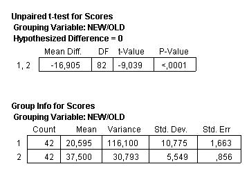
So the
mean difference between the scores for the Old and the New
menus is 16.905 points (the positive or negative sign only
depends on the arbitrary order in which we selected the
columns), and this is highly significant because the p-value
is very low.
We would
then express this as:
t(82)
= 9.039; p < 0.0001
And
if we want to know what’s going on with the means and standard
deviantions for the two groups, it’s all in the descriptive
statistics that StatView has given us in the second of the
above boxes.
A further
example may be borrowed from Tiina Puurtinen (1997), who
was interested in comparing the syntactic constructions
in translated vs non-translated children’s literature.
Puurtinen
constructed two corpora, one of Finnish originals, the other
of translations from English into Finnish. She then took
10 passages of 2000 words each from both corpora and counted
the numbers of nonfinite clauses. The mean numbers of nonfinite
clauses were then calculated for the two corpora, and these
means were compared using a group t-test.
When
I feed similar values into StatView (putting all the scores
in one column, and using the second column for the nominal
variables 1 and 2, for Nontranslated and Translated texts
respectively), this is what I get:
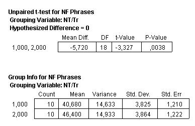
This
tells us that the mean difference of 5.72 is indeed significant,
since the p-value is well below the general threshold of
0.05. In Puurtinen’s own research we find p-values that
are indeed lower still (p < 0.01), so what she found
was more significant than what I found.
Group
t-tests assume that the two groups have a Normal distribution
(like a bell curve) and more or less the same degree of
grouping (standard deviation). It follows that when these
assumptions are not valid, the results of the test are not
particularly valid either.
This
is interesting when we look at the descriptive statistics
for the above examples (the numbers given in the second,
bigger boxes). In the case of the menus, the standard deviation
for the New menus (group 1) is about twice than of the Old
menus (group 2), so we might not feel very happy about using
a group t-test here (although with p < 0.0001 we perhaps
should not worry too much). In the second example, however,
the standard deviations of the two groups are very similar,
so we would feel the group t-test to be entirely appropriate
even despite the slightly higher p-value.
OUTLIERS
If we
do feel uncomfortable about big differences between the
standard deviations of our groups, there is often a simple
solution: shoot the numbers we don’t like.
This
means that, if our data show one or a few cases that are
clearly very different from the rest, at either the top
or the bottom of the range, we can decide that they have
no real reason to be in our sample, that they got there
by accident, that we are not very interested in them. And
then we eliminate them from our data.
In the
case of the menus, the New group has a bid standard deviation
because two menus that were so badly translated as to be
laughable. If these two menus are treated as outliers and
eliminated, the standard deviations become closer and our
group t-test seems a little more justified. Further, the
difference in the means of the two groups remains highly
significant:
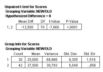 The elimination
of these outliers has the advantage of convincing us that
our result is not merely due to some accident in the sampling
process.
The elimination
of these outliers has the advantage of convincing us that
our result is not merely due to some accident in the sampling
process.
Of course,
we might also be genuinely interested in the outliers, if
only from a qualitative point of view. The high standard
deviation for the New group, with or without outliers, is
of interest for any hypothesis that would associate recent
developments of the translation market with relatively erratic,
uncontrolled performance and with a decline in collective
professionalism. This was indeed one of the qualitative
findings of the research.
WHAT
T-TESTS ARE MEASURING
T-tests
are not saying that a positive relation exists. They are
merely expressing the degree of certainty with which the
null-hypothesis (what we don’t want to find) can be rejected.
In the
menu example, p < 0.0001 thus means that there is very
little probability that the difference between the means
of the two groups is due to chance. We have not proved that
all menus produced in the 1990s are worse than all the menus
produced in the 1970s; we have not shown any causal relation
between the two variables involved; all we have done is
assess the probability that the mean differences between
our samples are due to chance.
If you
want to say more than that, you need more than these statistics.
CORRELATIONS
T-tests
are used when we hypothesize a patterned difference between
two variables or between two groups.
However,
if our hypothesis is that there is NO significant difference
between two variables, we are perhaps better off doing a
simple test of correlation.
This
is the case, for example, of the scores for the Language
and Culture errors in the menus. Here we are interested
in the possibility that a high Language score corresponds
to a high Culture score for the same menu. In other words,
when the value for one variable moves up or down, we would
like the value for the other variable to move up or down
accordingly.
This
moving up and down together is actually called covariance,
which can be measured as such. However the numbers given
for covariance analysis depend on the units used in the
measurement (measurements in Fahrenheit and Celsius will
give different covariance values). It is easier and more
meaningful to go straight to a correlation analysis.
To get
the correlation, put the scores into StatView and see what
it says.
Here,
for example, are the Language and Culture scores for seven
menus:
|
L
|
C
|
|
35
|
25
|
|
45
|
40
|
|
45
|
35
|
|
45
|
35
|
|
30
|
25
|
|
40
|
35
|
|
40
|
35
|
We want
to know if there is a good or bad correlation between these
variables. When we select the ‘correlation matrix’ test,
here is what we get:

Absolute
direct correlation is +1.0 (whenever one side goes up, so
does the other and to a corresponding degree); an absolute
lack of linear correlation would be 0.0 (no relation between
the up and down movements on either side); an absolute inverse
correlation would be -1.0 (whenever one side goes up, the
other goes down and to a corresponding degree). So here
we find the Language scores correlate absolutely with the
Language scores (which should be no mystery!) and that the
degree of correlation between the Language and Culture scores
is 0.891, which is high and thus a good indication of the
relation we were hypothesizing.
Correlation
matrixes can be done with more than two groups. So it is
a quick and easy way of seeing which variables move together.
SIMPLE
LINEAR REGRESSION
If the
correlation value 0.891 doesn’t mean much to us, we can
also visualize what is happening by drawing what is called
a ‘scattergram’ or a ‘scatterplot’. This means that one
variable goes on the x axis and the other on the y axis
(it doesn’t much matter which is where) and our scores are
then ‘scattered’ in accordance with these two dimensions.
For the above data on Language and Culture scores for seven
menus, this is what we get:

Each
of these points represents a menu, located so that we can
read off its score for Language (on the y axis to the left)
and for Culture (on the x axis at the bottom).
Clearly,
the higher the score for Language, the higher the score
for Culture. Which just means that there is a good correlation,
as we already know.
However,
we can go a bit further and ask StatView to draw a Bivariate
Regression Plot (in the Graph menu, under Analyze). And
here is what it gives us:
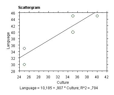
As you
can see, this is the basic scattergram plus a straight line
drawn through the points to indicate the best fit we could
hope for. This line is called the regression line.
Regression
lines of this kind are useful when we are trying to predict
values for data that we don’t have but could be assumed
to lie within the range of those we do have. For example,
we might be interested in predicting the Language score
for a menu with a Culture score of 32. By just looking at
the graph, we go from 32 on the x axis up to the line, mark
the point, and then go across to the corresponding Language
score, which would be about 39. You also get a formula to
do this:
Language
= 10.185 + 0.907 * Culture
So,
if we want to predict the Language score for a Culture score
of 32:
Language
= 10.185 + 0.907 * 32 = 39.209
The
numbers under the scattergram also include the R2 (r-squared)
value, which measures the amount of shared variance between
the variables, i.e. how much of the variance in x is accounted
for by y, or vice versa. This is in fact a measure of how
well the linear model fits the data. Here we are being told
that an estimated (^ means ‘estimated’) 79.4% of the variance
is accounted for by the data. Which is quite good.
This
kind of analysis is useful in cases where there is obviously
a lot of data missing but we still want to predict general
relations as far as possible.
For
example, we might test the hypothesis that the more publications
there are in a language, the less the percentage of translations
in that language (i.e. big languages translate proportionately
less than small languages). The problem here is that there
are a great deal of languages in the world but comparable
data are only available for about 20 of them (from Unesco).
So we can’t really do any sampling; we just have to assess
the possible correlation on the basis of the numbers available.
When we draw a bivariate regression for these two variables,
this is what we get (now from KaleidaGraph, because it’s
prettier and we can actually name the languages on the graph):
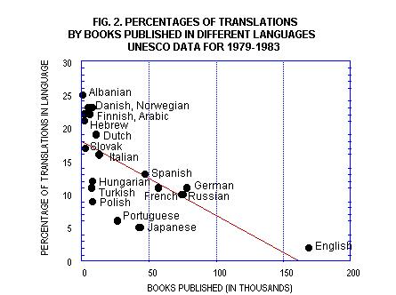
This
has been taken from Pym (1999). Here is the same thing from
StatView:
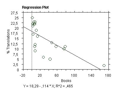 Since
StatView gives us the formula for the line, we could now
predict the translation rate for a language with a given
number of publications. For example, we know that Catalan
had about 2000 books published in 1980, so its x-value is
about 2, but there are no reliable data on the translation
rate at that time. We may now try to estimate that rate
as the following y-value:
y =
18.29 - 0.114 x 2 = 18.062
Since
StatView gives us the formula for the line, we could now
predict the translation rate for a language with a given
number of publications. For example, we know that Catalan
had about 2000 books published in 1980, so its x-value is
about 2, but there are no reliable data on the translation
rate at that time. We may now try to estimate that rate
as the following y-value:
y =
18.29 - 0.114 x 2 = 18.062
So we
would predict that Catalan had a translation rate of about
18% for 1980. How good is the prediction? Well, the only
figure I do have is an estimate of 16.5% for 1977, which
is at least close to our prediction. (The linear analysis
of these data is actually more useful as a check on people
who argue that the English language actively excludes translations,
when its low rate could be due to no more than its high
number of publications.)
The
R2 here is 0.465, which means that only about 46% of the
variance is accounted for by the data. This is a little
below the 50% that might make us feel confident.
Like
t-tests, this kind of test assumes that the data have about
the same variance in the two groups. In our example this
is a risky assumption, since the standard deviation for
the Books variable is about 40, and that of the %Translations
variable is around 8. This sort of difference suggests that
the relation is in fact far from linear.
References
Fallada,
Carmina. 1998. ‘Are
Menu Translations Getting Worse? Problems from the Empirical
Analysis of Restaurant Menus in English in the Tarragona
Area’.
Puurtinen,
Tiina. 1997. ‘Syntactic Norms in Finnish Children’s Literature’.
Target 9:2. 321-334.
Pym,
Anthony. 1999. ‘Two
principles, one probable paradox and a humble suggestion,
all concerning translation rates into various languages,
particularly English'
Wright,
Daniel B. 1997. Understanding Statistics. An Introduction
for the Social Sciences. London, Thousand Oaks, New Delhi:
Sage.
Last
update 13 January 2000
|